Naive Bayes Classifier: Concepts, Examples and Code

Naive Bayes Classifier

Naive Bayes models are extremely fast, very simple and highly suitable for high dimensional datasets. The reason behind this is there simplicity and very less tunable parameters. This tutorial will cover the following sub topics and explain everything with a suitable and understandable examples. if you are a beginner this tutorial is for you. You can check the list of topics given below and start from where ever you want. 

In this tutorial we have set following few agendas to discuss. 

a) Bayesian Theorem
b) Proof of Bayes Theorem
c) Example on Conditional Probability
c) Bayesian Classification
d) Weather Dataset Example
e) Python code to understand Gaussian Naive Bayes classifier
f) Python Coding Exercise on Iris Data Set
g) When should you use Naive Bayes Classifier

Bayesian Theorem

This is one of the most important theorems in the theory of probability and statistics. It describes the relationship of conditional probabilities of statistical quantities. The theorem finds the probability of an event given the probability of another event that has already occurred. Bayes theorem is stated as follows:

 Here, P(A|B) is read as probability of event A given that B is true. It is also called as posterior probability, P(B|A) is the likelihood. P(A) is called Priori and P(B) is called marginal.

Proof of Bayes Theorem

Before we move forward lets give proof  of the above equation.

We know that:

From (1) and (2) we can say that 

Let us understand conditional probability with an example first. 

Example 1 Conditional probability

Let us assume we have a bag which contains 3 Red apples, and 2 green apples. Two apples are drawn without replacement. Find the probability that both of the apples are green.

This example is based on conditional probability:

 Event A:

     P(Green)=2/5=0.4

Now when the event A has happened we are left with 4 apples in the bag {No replacement}

Event B:

    P(Green | A )  = 1/4=0.25, Which is the probability of Green when the event A has already occurred.

Now lets find the probability of both these events take place and solve by the formula also

P(A intersection B)=2/5*1/4=1/10=0.1

           P(A|B)=0.1/0.4 =0.25

Bayesian Classification

In Bayesian Classification we are interested in finding the probability of a class or Label given some observed features. Which can be written as P(Label | Features). Bayesian theorem can show how we can compute this directly as follows

                              P(Label | Features)=(P(Features| Label)*P(Label))/P(Features)

Weather Data Set Example

Lets us understand this concept by solving a problem with Bayesian classification. This problem of a weather dataset can be seen in  many books of data mining and machine learning.

We are given with 4 input features Outlook, Temperature, Humidity and Rain. We are given a label called Play cricket which can have two values Yes or No. we are asked to tell weather we should play cricket Today when the  outlook is Sunny and Temperature is Hot. Lets try to predict this.

	Outlook	Temperature	Humidity	Rain	Play cricket
1	Rain	Hot	High	True	No
2	Rain	Hot	High	False	yes
3	Overcast	Mild	High	False	Yes
4	Sunny	Cool	Normal	False	Yes
5	Sunny	Cool	Normal	True	No
6	Sunny	Cool	Normal	True	Yes
7	Overcast	Mild	High	False	No
8	Rain	Cool	Normal	False	Yes
9	Sunny	Mild	Normal	False	Yes
10	Rainy	Mild	Normal	True	Yes
11	Overcast	Mild	High	True	Yes
12	Overcast	Hot	Normal	False	Yes
13	Sunny	Mild	High	True	No

Lets do some computations on our weather dataset. P(Features | Label)

P(Outlook | Play Cricket)

                   Outlook

	Yes	NO	P(Yes)	P(No)
Sunny	3	2	3/9	2/5
Overcast	4	0	4/9	0/5
Rainy	3	2	3/9	2/5
Total	10	4	-	-

 Here, we will search in the above weather data set the corresponding values. For example {When Outlook is sunny, Number of 'Yes' in Play cricket are  3  } That is why the column {Sunny, Yes}=3  Similarly column

  {Sunny, No}=2  ,P(Yes) = P(Sunny when Play cricket=Yes)/Total Yes in Play Cricket  Similarly P(No)=P(Sunny when Play Cricket=No) /Total No in Play Cricket        

                       Temperature

	Yes	No	P(Yes)	P(No)
Hot	2	2	2/9	2/5
Mild	4	2	4/9	2/5
Cool	3	1	3/9	1/5
Total	9	5	-	-

 Similarly  we have calculated the values for the Temperature table.

                        Play Cricket

	Play Cricket	P(Y)
Yes	9	9/14
No	5	5/14
Total	14

We can see in the play cricket column that the number of rows with value 'YES' are 9 and the number of rows with value 'NO' are 5. P(Y) computes the corresponding probabilities.

The same tables are to be made for other two features which are Humidity and Rain. Lets perform some predictions with this much of the information.

Example: Suppose we are told that the weather today is Sunny (Outlook) and Temperature is Hot Should we Play cricket or not. Lets predict that with Bayesian Classifier.

P(Sunny , Hot)

Lets find the probability of Yes first

P(Yes | Today)=P(Sunny | yes)*P(Hot | yes)*P(Yes) / P(Today)

Consult the above tables to find out the corresponding values of the terms

P(Sunny | yes)=3/9, P(Hot | yes)=2/9, P(Yes)=9/14

Let us Skip the P(Today) because its in both terms

P(Yes | Today)=3/9*2/9*9/14=.031

Now lets find the probability of No now

P(No| Today)=P(Sunny | no)*P(Hot | no)*P(no) / P(Today)

P(No | Today)=3/5*2/5*5/14=0.0857

Let us normalize the values

Normalize=0.031/0.031+0.0857=0.27

Which means that P(Yes | Today)=0.27=27%

Then P(No | Today)=1-0.27=0.73=73%

The probability of No cricket =73%

So the prediction is NO cricket.

Question:  Predict the probability of play cricket if  outlook is rainy, temperature is mild, humidity is high and rain is false?

             Hint { Compute 2 other tables Humidity and Rain also so that you have all the 4 tables available which are needed to solve this question}

Python code to understand Gaussian Naive Bayes classifier

Now we are ready to do a python coding exercise to implement Naive Bayes Classifier. We are going to implement Gaussian Naive Bayes Classifier in the code below. This is the simplest one you can use other naie bayes classifiers also. It assumes the data from each label is drawn from a simple Gaussian Distribution. Lets consider the following data created through the code.

One simple way is to assume that the data is described by a Gaussian Distribution with no covariance between the dimensions. We can fit this model by simply finding the mean and standard deviation of the points within each label, which is all we need to define this distribution.

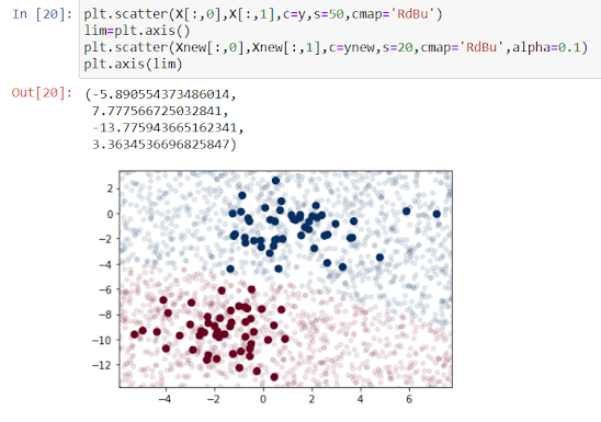
Lets implement this model with sklearn package as shown below. Lets also generate some new data and predict the label. GaussianNB is the Gaussian Naive Bayes Classifier

Lets plot this new data to get an idea where the decision boundary is.

In the classification we can see a slightly curved boundary.  The boundary in Gaussian Naive Bayes is quadratic.

Python Coding Exercise on Iris Data Set

Lets do one more python exercise on famous Iris dataset. It contains 150 samples of three species of flowers which are Iris virginica, Iris setosa and Iris versicolor. There are four features of the dataset given as shown below. SEPEL_LENGTH, SEPEL_WIDTH, PETAL_LENGTH and PETAL_WIDTH in centimeters. This dataset is available on sklearn package. On the basis of these input features we predict the type of the flower i.e. Iris virginica, Iris setosa and Iris versicolor. You can also download this data set online from this link Iris Flower Dataset | Kaggle

Lets use Naive Bayes Classifier on this data set

Firstly, let us import the necessary libraries like pandas, numpy and sklearn first. Then we load the dataset which is present in sklearn package, so we simply load it from there. You can also download the dataset from the link above and load it into your python notebook . Iris.data shows the values of the features. We have shown only few of the rows here.

Let us assign data to X and the target value or label to y. X.shape is the number of rows that is 150 which is the total number of flowers in the dataset. The number of column or features are 4 and the target value consist of 150 values and the value is either  Iris virginica, Iris setosa or Iris versicolor ie the flower type.

Let us split the data into train and test sets as follows. we will use sklearn package and import train_test_split()  to perform this function.

In the next cell we have imported the Gaussian Naive Bayes classifier and used it to fit our train data and in the last cell we have stored the predicted value and then used the accuracy_score() function to find the accuracy of our model.

 

You can import other naive bayes classifiers like multinomial Naive Bayes and see the results. 

When Should You Use Naive Bayes algorithm

It is often a good choice as an initial baseline classifier. If it performs well then great otherwise you should explore some more sophisticated models. Some of the advantages of Naive Bayes are as follows:

 1) They are extremely fast for both training and prediction

 2) They are often very easily interpretable

 3) They have very few tunable parameters

 4) They are very easy interpretable